An overarching concern in snow hydrology is the spatial distribution of snow water equivalence (SWE). Our ability to utilize spatially distributed models of snowmelt and runoff is limited by our ability to adequately characterize the spatial distribution of SWE. We will present a study of an alpine basin in Colorado for which a DEM is available and the major landscape types have been mapped and digitized onto a GIS. Using a combination of field measurements and geostatistical techniques we have estimated the distribution of snow water equivalent throughout the basin and compared it to the mapped landscape types, to investigate the relationship of snow water equivalent to landcover type, slope, and aspect.
One of the most challenging problems in snow hydrology is understanding the spatial distribution of snow water equivalence (SWE) in montane catchments. A number of researchers have shown that the spatial distribution of SWE is influenced by a number of factors in a non-linear fashion, including slope, aspect, elevation, wind redistribution, terrain features, and vegetation type and amount. Consequently, understanding the spatial distribution of SWE from first principles has had little success.
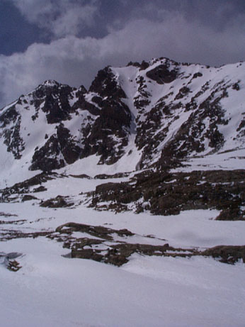
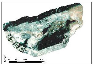
Alpine areas are particularly problematic for understanding the spatial distribution of SWE. Avalanches, sloughing from steep terrain, wind redistribution, variation in solar radiation, and other variables have a much greater influence on the spatial distribution of SWE in alpine catchments than downstream forested catchments because of the lack of vegetation to intercept, accumulate, and shelter snow. Moreover, alpine catchments are a mosaic of areas with and without snow because of the importance of redistribution processes (Figure 1), further complicating our understanding of the spatial distribution of snow. Hence our understanding of the spatial distribution of SWE is rudimentary at best in alpine terrain.
The spatial distribution of SWE is generally measured by collecting point measurements of snow depth and density using samples extracted from snow pits. Determining the location of these point measurements has generally been done using a combination of topographic maps and aerial photographs. The method is tedious, laborious, and time-consuming, with uncertainty in the location on the order of 10's of meters. Recent technological advances in Geographic Information Systems (GIS) and Global Positioning Systems (GPS) may provide the key for increasing our understanding of the spatial distribution of SWE in alpine catchments. Fast, efficient, and accurate retrieval of point measurements of the properties of SWE using GPS may allow efficient transfer of the information to a GIS and then the ability to test the dependence of SWE on independent variables such as landscape type, slope, and aspect.
Here we combine the use of GIS and GPS at a high-elevation catchment in the Front Range of the Colorado Rockies to investigate: (1) the advantages and disadvantages of two different GPS models for identifying the location of point measurements of snow depth; (2) the combination of the GIS and GPS information to determine if there is a relationship between basin properties such as landscape type, slope, and aspect, and the spatial distribution of SWE; (3) the use of kriging techniques for spatially distributing the point measurements of SWE to evaluate the effectiveness of the kriging method; and (4) methods of improving our estimate of SWE in alpine basins.
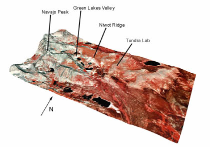
The Green Lakes Valley is an east-facing headwater catchment that abuts the Continental Divide and is located entirely within the Arapaho-Roosevelt National Forest. The Green Lake 4 basin ranges in elevation from 3575 to 4000 m, is 224 ha in size, and appears typical of alpine basins in the Colorado Front Range (Figure 2). The area has a continental climate, receiving about 1000 mm of precipitation annually, 80% as snow. Niwot Ridge forms the northern boundary of Green Lakes Valley and is an UNESCO Biosphere Reserve and a Long-Term Ecological Research (LTER) network site.
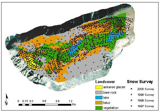
As part of the (LTER) program, a snow survey was performed at maximum accumulation in the Green Lakes 4 watershed from 1997 through 2000. Snow depths were measured using hand probes. The spatial density of snow depths was nominally 50 m between sample points. However, the spatial density of field measurements varied from year to year as a function of the number and experience of field personnel. Each data point was registered using a GPS and transferred to a 10-meter Digital Elevation Model. Snow density was measured at fewer sites because the density of snow is less variable than snow depth. The SWE was then calculated as the product of snow depth and density.
A Trimble Pro XR Integrated GPS/Beacon Receiver with a TDC1 data logger was used to collect the position and attributes (snow depth) of points within the Green Lakes Valley during the 2000 snow survey. Using the Omnistar Real-Time Differential Correction Service, the data were real-time corrected while being collected in the field. The real-time correction results in a nominal horizontal accuracy of <0.6 meters for the data collected. Snow depths and associated comments were entered into the data logger using a Trimble Data Dictionary that was created before the survey was conducted. The raw data collected were downloaded and post-processed/differentially corrected within Pathfinder Office 2.51 software package. The data were post-processed due to the fact that on occasion the RTCM signal was lost and the post-processing increases the accruacy of such points. The post processing data were retrieved from the Compasscom, Inc. Base Station in Denver, 35 km away from the study site. The processed data were then exported to an Arc/Info generate format where the AML script created by Pathfinder Office was used to create a point coverage.
The accuracy of the Trimble comes at a cost. The size and weight of the GPS unit can be cumbersome in the field. The Trimble is a multiple piece unit including the data logger and the receiver. The total weight with batteries is 1.84 kg (4.07 lb) while the dimensions are the TDC1 data logger 20.8 cm x 8.9 cm x 4.5 cm and the Pro XR 11 cm x 5.1 cm x 19.5 cm. There is a large monetary cost as well, the Trimble Pro XR along with the TDC1 data logger retails for $11,000. The battery life was found to be approximately 4 hours, which means multiple batteries must be carried into the field, which adds an extra 0.71 kg (1.56 lb) to the total weight.
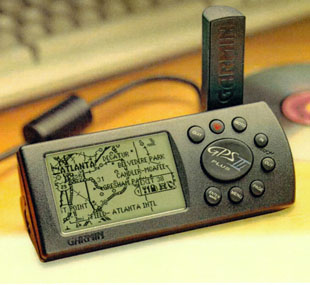
During the survey, we evaluated the lighter and less expensive Garmin GPS-III Plus. Waypoints were collected with the Garmin in the same location as points recorded with the Trimble. The raw data were downloaded to the PC using the program GPSdb which was downloaded from the Internet. The optional Garmin GBR 21 DGPS receiver was not used, therefore there was no differential correction applied. The accuracy of the Garmin according to the factory specifications is 15 meters. The raw data were exported as a DBF file and a point coverage was generated using ArcToolbox 8.1.
The Garmin is significantly smaller than the Trimble unit. The unit weighs 255g (0.56 lb) and the dimensions are 5.9 cm x 12.7 cm x 4.1 cm. The weight is less than a single Trimble external battery. The battery life was found to be about 6 hours, which is a significant improvement over the Trimble batteries. The unit's retail price is under $300. There is a significant benefit in size, weight, battery life, and retail cost of the Garmin with respect to the Trimble ProXR.
 (a)
(a)
 (b)
(b)
The DEM was developed by Analytical Surveys, Incorporated (ASI) in Colorado Springs. The DEM and corresponding digital orthophotos are for a 10.5 km (E/W) by 5.4 km (N/S) area that encompasses the Mountain Research Station, Niwot Ridge, Green Lakes Valley and the Continental Divide (Figure 1). The DEM was developed from 1:12,000-scale black and white aerial photography used to collect breaklines and mass points in the Green Lakes Valley area where any feature larger than 10 meters was captured. Then 1:24,000-scale Color Infrared (CIR) aerial photographs were utilized for feature capture on Niwot Ridge, and 1:40,000-scale CIR aerial photographs were used to fill in the study area margins. Breaklines and mass points were collected at a coarser resolution as photograph scale decreased. Digital orthophotos were generated from all three scales of photography.
The GIS software used for the manipulation and analysis of the data was ESRI's ArcInfo. The data are stored in ArcGIS coverage, grid, and TIN formats. ArcInfo 7.0.2 Workstation for Solaris and ArcInfo 8.1 Desktop and Workstation for Windows NT were the primary software packages used. The Spatial Analyst and Geostatistical Analyst extensions were used for grid analysis and kriging.
An attribute of SWE was calculated within ArcMap by multiplying the point snow depths by the average density of the snow, determined from snow pits. The point information on SWE was interpolated over the basin using spatial kriging. Ordinary Kriging with the exponential model was performed with the Geostatisical Analyst extension, which used the following equation: 0.39214*Exponential(183.43)+0.28408*Nugget.
The development of landscape coverages is illustrated in Figure 4. The aerial photographs (Figure 4a) were overlain on the DEM (Figure 4b). Landcover type was then mapped in the field using expert knowledge in combination with the aerial photographs and DEM. Bare rock makes up 29% of the basin area, talus 33%, vegetated soils 29%, the Arikaree glacier 4%, and there are two lakes in the basin (Figure 4c).
 (a)
(a)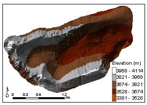 (b)
(b)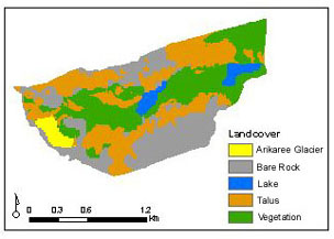 (c)
(c)Snow depth measurements at maximum snow accumulation were conducted from 1997 to 2000. The number of snow depth measurements ranged from 193 measurements in 1997 to 751 in 2000 (Figure 5). A problem is how many and where to add zero points on snow-free terrain that was too steep to sample. We've added zero points at 50-meter intervals, our nominal sampling density, to our 2000 snow survey data.
Data points collected with the Garmin GPS were compared to the real-time differentially corrected data collected with the Trimble. Fourteen data points were recorded with each GPS unit at 50 meter intervals within the basin. In order to compare the accuracy of the Garmin, the data from the Trimble are assumed to be the true coordinates. The mean distance between corresponding points recorded with each unit is 3.9 meters, with a standard deviation of 1.3 meters. The coefficient of variation was found to be 33.7%. With a mean difference of 3.9 meters, the Garmin exhibited a higher accuracy than the nominal 15 meter accuracy.

The Garmin is limited by a few factors relative to the Trimble. Unlike the Trimble, the Garmin does not have the option of masking out measurements when the Dilution of Precision (DOP) is above a preset threshold. Although comments may be added to each measured point with the Garmin, it is difficult to enter text since each character must be entered by scrolling through the alphabet.
In all years, snow depth was greatest on the Arikaree glacier and then on talus (Figure 7). Snow depth was generally similar on bedrock, vegetation, and lakes, and always less than on the Arikaree Glacier and on talus. To illustrate, in 2000 (Figure 7) mean snow depth was 5.11 meters on the Arikaree glacier, 2.17 meters on talus, 1.47 meters on rock, 1.40 meters on vegetation, and 0.8 meters on water. Over the four years, talus fields generally had about 50% deeper snow than vegetation, rock, or lakes. A plot of the cumulative distribution function of snow depth by landscape type provides a nice visual presentation of the differences in snow depth by landscape type (Figure 8a). For example, talus areas always have greater snow depth than vegetated areas and rock areas below 80% percentile.

Our results show that the spatial distribution of snow depth in alpine catchments is influenced in part by landscape type. The correlation between snow depth and landscape type suggests that we can improve our estimate of the spatial distribution of SWE in alpine catchments by incorporating landscape type as a proxy variable.


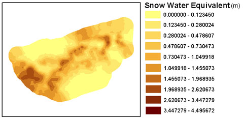
There is a qualitative agreement between the kriged SWE values and expert knowledge of the basin (Figure 9). For example, the deepest snow depths are located at the Arikaree Glacier. However, more quantitative measures suggest that the kriged data underestimates the amount of SWE in the basin. The best unbiased estimate of SWE for areas where the snow depth point sample size is greater than 200, is to multiply the average snow depth in the basin by the average snow density, and multiply that value by the area of the basin. The amount of SWE in the basin using this method is 2.175 x 10⁶ m3 of water. The kriged estimate is 40% lower at is 1.307 x 10⁶ m3 of water.
The cumulative distribution function of kriged snow depth by landscape type provides some explanation (Figure 8b). The cumulative distribution function of kriged snow depth values has a smaller range when compared to the measured values (Figure 8a). For example, measured snow depths for talus areas ranged from 0.2 to 10 m. In contrast, kriged values of snow depth from talus areas ranged from 0 to 5 meters. Moreover, 40% of the measured snow depths for talus were greater than 3 m. However, after these values were kriged, only 15% of the snow depths in talus areas were greater than 3 m. Kriging results in a loss of the larger values for snow depth. Thus, the smoothing function inherent in spatial kriging appears to result in an underestimation of SWE in this alpine basin.
The accuracy of the Garmin was found to be sufficient for snow surveys. The lower cost, lighter weight Garmin may be preferred over the heavier, bulkier, battery-demanding Trimble. However, the ability of recording attributes must be improved for data management purposes in order for the Garmin units to move from recreational use to use as a data collection tool.
The combination of GIS and GPS allows for the testing of the dependence of SWE on parameters such as landscape type. Further exploration with interpolation models that incorporate factors such as landcover type should be evaluated. The 40% underestimate of SWE using kriged surfaces needs to be investigated in order to determine what is the best estimation of SWE: modeled (e.g. kriging) or measured values.
Thanks to the many students, field staff (especially T. Bardsley), Matt Tomaszewski, and volunteers who have helped with the snow surveys over the years.
This research was funded by NSF EAR-9526875 (Hydrology), Army Research Office grant DAAH04-96-1-0033, NASA-EOS, and the Mountain Research Station of INSTAAR and CU-Boulder. Ongoing maintenance and data access is funded by the NSF grants DEB 92-11776 and DEB 98-10218 to the NWT LTER project.