SNOW HYDROLOGY (GEOG 4321): STATISTICS: 1999

Instructor: Eran Hood

Telephone: 492-4279 or 492-4815

Statistical Topics

1. The sample mean of a set of n measurements is the sum of these measurements divided by n.

2. The standard deviation (s) of a set of n measurements is a measurement of the variability in the data. For a normal distribution, 68% of the data lie within 1 standard deviation of the mean and 95% of the data lie within two standard deviations of the mean. The standard deviation is calculated by the following equation:

3. The standard error (S.E.) describes the variability that can be expected in the means of samples by repeated random collection from the same population. The standard error is computed by dividing the the standard deviation by the square root of the number of measurments. In other words, the standard error will be reduced by increasing the sample size.

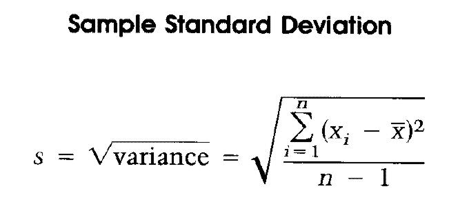
   S.E. = s/ square root n

   where s is the standard deviation and n is the number of samples

4. Regression Analysis concerns the study of relationships among variables for the purpose of constructing models for prediction and other inferences. We can study the relationship between two variables x, the independent variable, y, the dependent variable, in order to be able to predict y from x. A good first step is to plot a scatter diagram of the observations in order to make a visual analysis of the relationship between the two variables.

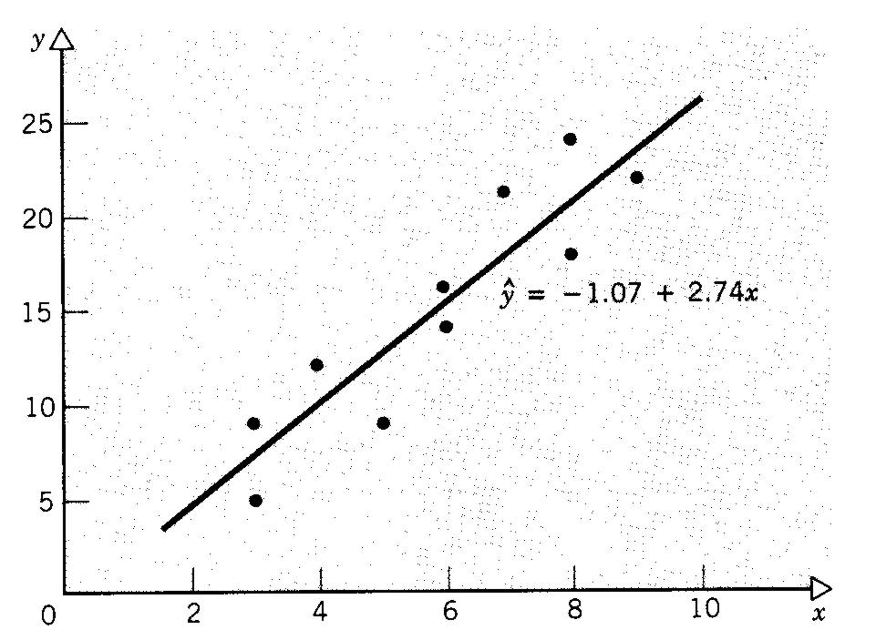
   Using a standard statistical package, you should fit a line to the data. This should be done by performing a simple linear regression. The resulting least squares regression line is a best-fit line based on the positions of the data points. The "goodness of fit" of the line is described by the r-squared term such that an r-squared of 1.0 is a perfect fit to the data and an r-squared of 0.0 means there is no relationship between x and y. Another way to think of this is that an r-squared of 0.95 means that x explains 95% of the variability in y.

   The least squared regression line can be described by the equation: y = b + mx, the standard equation of a line where b is the y-intercept and m is the slope of the regression line. In many statistical packages, m and b can be found under the heading "coefficients" in the regression output file; b will be the coefficient for the intercept and m will be the coefficient for the x variable.

   In order to determine whether the relationship between two variables is significant it is important to look at two values, the r-squared and the "P-value" of the slope of the line. In the case of the r-squared, values closer to 1.0 indicate a significant relationship while values close to 0.0 do not. In the case of the P-value, you want a very low number. A P-value for your slope which is less than 0.05 indicates that you are more than 95% confident in the relationship between the two variables. Similarly, a P-value of less than 0.01 indicates that you are more than 99% confident in the relationship between variables. Often a high r-squared value will lead to a P-value which is much smaller than 0.01 if you have a good number of samples.

5. The paired t-test is useful for testing hypotheses about the equivalency of two samples ( in our case data collected at snow courses vs data collected at SnoTel sites). To start, pair the data from the two sources by placing them in columns next to each other. Now calculate the difference between each pair. From these differences between your pairs, you can calcualte a mean difference between the two data sets. Next, calculate the std deviation and std error for the differences. For the t-test, calculate a t-statistic by dividing the mean of the differences by the std error of the differences. To evaluate the t-statistic, it is necessary to look at a T-table which displays critical values for t based on sample size and probablilty level. In our case, find a critical value for t with 10 (n or sample size - 1) degrees of freedom and a significance level of 5% or 0.05. If your t-statistic is greater than the critical value, then it can be assumed that the two measurement schemes are significantly different. Conversely, if the t-statistic is less than the critical value from the table, then it can be assumed that the two measurement schemes are equivalent.