SNOW HYDROLOGY (GEOG 4321): SNOW DISTRIBUTION

Instuctor: Mark Williams
Telephone: 492-4794 or 492-8830

Alpine (Tyler's stuff)
Harvesting forests for water yield

Problem Statement

• The major source of water supply for runoff and groundwater recharge over wide areas of the mid-latitudes is snowmelt from seasonally snow-covered areas of the Earth's mountain ranges.
• For example, in the western United States, while episodic snowfall events produce widespread shallow snow cover of short duration, mountain snowpacks are typically much deeper, and store and release water well into the spring and summer.
• There is a need to
  1. Understand and predict the timing, rate, and magnitude of snowmelt runoff under current climate conditions.
  2. To predict potential snowmelt responses to changes in climate.
  3. The increasing need to understand intrabasin snowmelt characteristics for environmental analysis of such factors as basin ecology [Baron et al., 1993], water chemistry [Wolford, et al., 1996] and hillslope erosion [Tarboton et al. 1991].

Background

• Little work done at the process-level.
• Most work done using index snow courses with gentle terrain that do not represent mountain environments.
• Some work has been done with SWE as a function of elevation.
• However, the relationship between SWE and elevation breaks down in mountain areas because of snow redistribution by wind.
• Why so little work done on snow distribution in high mountains:
  1. Hard to get to; many mountain roads closed in winter.
  2. Dangerous: cold, wind, avalanches, etc.
  3. These conditions make for difficult working conditions, also hard on equipment.
  4. Hard on equipment: temperature extremes; temperature changes across 0 deg C result in condensation in electronics.

Snow Distribution Parameters

Overview of parameters

• Slope.
• Aspect.
• Elevation.
• Surrounding terrrain (view factor).
• Reflected energy from other surfaces.
• Long-wave emission from cliffs, etc.
• Wind fetch.

Snow properties that vary with time and space

• Depth.
• Density.
• Temperature.
• Chemistry.
• Rate of change (eg snowmelt).

Controlling factors

1. Snowfall amount (intensity, duration)
   • Elevation.
   • Slope Angle.
   • Windspeed.
2. Redistribution
   • Erosion in areas of convergent flow.
   • Deposition in areas of diverging flow.
3. Avalanches, sloughs
   • Changes spatial distribution of snow.
   • 30-60% of alpine snow cover transported by avalanches in the Caucasus Mountains.
   • Increase or decrease melt rate.
   • Often results in deeper snowpacks which provide meltwater late into the melt season.
4. Ablation
   • Sublimation and evaporative losses from snow surfaces, interception in trees, etc.
   • Ground melting.
   • Snowmelt.
   • Differential snowmelt during mid-winter, eg snowmelt on south-facing slopes, but not north-facing slopes.
   • Differential energy balance throughout basin.
5. Elevation
   • Generally get increased orographic precipitation with increasing elevation in mid-latitude mountains.
   • Below treeline often get increased SWE with increasing elevation.
   • Above treeline, wind redistribution supercedes the elevation effect such that there is little if any correlation between elevation and SWE.
6. Topographic effects
   • Static parameter that affects all of the above.
   • Topographic affects are mediated by processes such as blowing snow, avalanching, differential energy balance, etc.

Scales of Interest

Effect of Topography

Effect of Vegetation

Forested Environments 1

Forested Environments 2

Open Environments

Relative Accumulation Rates

SPATIAL SAMPLING

Hydrologists typically want to estimate the total volume of water delivered to a given area, such as a catchment, for some time period. Almost always, we have very limited and discrete gauge measurements that we must somehow distribute over the region of interest. Given point values for any measure (air temperature, nitrate in grounwater, elevation, etc) it is often desireable to create a grid that "fills in" the values between the points. Not a simple thing to do as it turns out.

Things to consider.

• what is the distribution of the points across the surface?
• does the surface have to fit exactly to the points? (noisey or not)
• how much smoothing is desired?
• how much complexity of the surface is desired?

• We can represent the area of the catchment by the rectangular coordiates x and y.
• A is the catchment area
• P is the total precipitation amount
• p(x,y) is the precipitation amount at each point, so
• 
• However, this is way hard to solve. So we use various analytical methods.

WEIGHTED AVERAGES

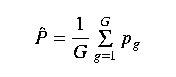
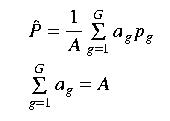
Direct-weighted avearge methods use the general equation

• 
• where g is an individual gauge
• G is all the gauges
• v_g are weights such at
• 

Arithmetic average In the arithmetic average method, each gauge is assigned the same weight of 1/G. The regional average therefore becomes the arithmetic mean of the values measured at all the gages in the region

Thiessen Polygon The region is subdivided into G subregion, each subregion approximately centered on each of the G gauges. The key is that subregions are closer to their central gages than they are to other gages. Thiessen in 1911 developed a method for delineating the boundaries of the subregions that are closest to each of the G gauges.

SURFACE FITTING

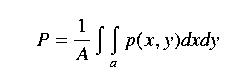
Surface fitting methods are used to represent precipitation at all points of the region of interest. This method is really a model of the spatial variability of precipitation (storm, max snow accumulation) that can be depicted on a map.

• Interpolation: spatial variability of precip mapped such that the precip at a gauge point has to equal the gauge measurements. The spatial variability is forced through the measurment points.
• Smoothing: modeled precip surface does not have to match measured ppt at a gauge
• Statistical (Stochastic): minimize estimation variances at ungauged points
• Deterministic: model precip at ungauged points using best knowledge

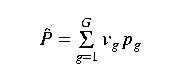
General procedurs. A grid covering the region of interest is established. The grid spacing is at the discretion of the analyist but usually about 1/10 the average distance between gauges. The total number of grid cells is J and each grid is j. Values of precipitation at each point j are estimated from the measured values:

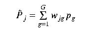
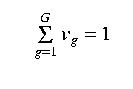
where p hat j is the estimated precipiation at the jth point, p sub g is the precip measured at gauge g, and w sub jg is the weight assigned to station g for grid node j. To ensure an unbiased estimate of P, most methods constrain the sum of the weights for each point as

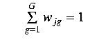
Most contouring routines use only the p sub g within a certain radius around a grid cell j to estimate p hat j, with w sub jg = 0 for all measured values outside that radius. The essential differences among rountines are how the weights w sub jg are established.

Isohyetal Method. Draw contours of equal precipitation depth.

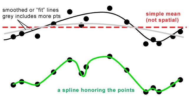
Least squares. Similar to the isohyetal method, except that the weights are determined by fitting a trend surface to the measured values such that the error (M) is minimized:

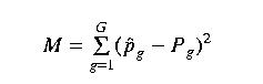
This surface is expressed mathematically as a polynomial in x and y, the coordinates of the system. This equation establishes the value of the coefficients of the polynomial, resulting in the least-squares name. You can use lots of terms in the polynominal, and as the number of terms increases, the surface fits the measured terms more closely. However, the increasing fit often comes with unwarranted and meaningless zones with little connection to reality.

Spline-Surface Method. A spline surface is similar to the least squared method. However, it finds the surface with minimum curvature that fits exactly through the measured values. It is computationally burdensome. However, that is no longer a problem with todays computational power.

Inverse-Distance Interpolation. Interpolation of the weights are a function only of the distance between each of the J grid points and each of the G gauge locations. Inverse distance weighting is the simplest interpolation method. A neighborhood about the interpolated point is identified and a weighted average is taken of the observation values within this neighborhood. The weights are a decreasing function of distance. The user has control over the mathematical form of the weighting function, the size of the neighborhood (expressed as a radius or a number of points), in addition to other options.

The simplest weighting function is inverse power:

The neighborhood size determines how many points are included in the inverse distance weighting. The neighborhood size can be specified in terms of its radius (in km), the number of points, or a combination of the two. If a radius is specified, the user also can specify an override in terms of a minimum and/or maximum number of points. Invoking the override option will expand or contract the circle as needed. If the user specifies the number of points, an override of a minimum and/or maximum radius can be included. It also is possible to specify an average radius based upon a specified number of points. Again, there is an override to expand or contract the neighborhood to include a minimum and/or maximum number of points.

Kriging. Kriging or optimal interpolation is a general term for a group of statistical methods in which the weights are derived by minimizing the variance of the interpolation error. Kriging uses known values and a semivariogram to determine unknown values. It was named after D. G. Krige from South Africa. The procedures involved in kriging incorporate measures of error and uncertainty when determing estimations. Based on the semivariogram used, optimal weights are assigned to unknown values in order to calculate unknown ones. since the variogram changes with distance, the weights depend on the known sample distribution.

Here's an example of Inverse Distance Weighting using the Yellowstone Snow-Elk project.

Hypsometric.

Conceptually, the hypsometric method is a deterministic, smoothing, surface-fitting mehtods. The method is appropriate for regions in which orographic effects are important, so that the precip of interest is a strong function of elevation. A contour map of topography is required to apply the method.

First, plot the measured p sub g values against elevation of that station (z sub g). Establish a relationship between precipitation and elevation, the orographic equation:
p hat (z) = a + bz
This relationship may vary systematically within a region; windward versus lee slopes of a mountain range for example.

Second, relate elevation (z) to the area above a given elevation (A sub z), called a hysometric curve.

Next,

• select an elevation interval, delta Z, and divide the total elevation range into H increments of delta Z.
• From the hypsometric curve, determine the fraction of the total area within each increment of elevation; designate these fractions as a sub h, h = 1, 2, ...H.
• Use the orographic equation to estimate the precipitation at each elevation interval z sub h, where z sub h is the central elevation of each elevation increment.
• Compute the estimated areal average precip as

  

Back to Course Content